Logical Volume Management

Before I start explaining Logical Volume Management (LVM), I would like to briefly talk about why I wrote this post and what it covers. Although there are many articles about LVM on the internet, I noticed one thing while researching this topic. Some of the articles weren’t explanatory or comprehensive enough. This is why I wanted to gather what I’ve learned into this article, explaining it as a complete whole, starting from physical disks, which are the foundation of this subject, all the way up to its top layer. First, we’ll take a look at a situation that arises in a system without LVM. After this, I will explain what LVM is and describe its structure by showing how it solves this situation. Then, I’ll go over the other advantages of LVM.

Log Files Filling Up the Disk

First, let’s look at what happens in a system without LVM when the storage space fills up. The output of the system’s lsblk command looks like this:

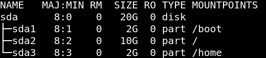
In the attachment below, there’s a newly added 20 GB storage device, /dev/sdb, in the system. This storage device has been partitioned into 10 GB sections as /dev/sdb1 and /dev/sdb2. These two partitions, mounted at /data1 and /data2, were created to store the applications’ log files.

Let’s simulate one of the problems encountered in real life: log files consuming the disk’s space. Since this command will fill up the disk quickly, don’t try it on your own systems.

cat /dev/zero > /data1/application.log cat /dev/zero > /data2/application.log

In the diagram below, you can more clearly see a system without LVM and the operation we performed using the watch df -h command. We’re simulating log files consuming the disk’s space, and the disk starts filling up after this command.

In this situation, you could of course choose to move the log files to another disk or delete them. But as you can probably guess, this process gets harder as the number of disks increases. In this case, you could expand your file system using LVM, or solve this problem in other ways. However, since the system you see above doesn’t use LVM, you can’t expand your file system. Now I’ll explain LVM, which solves this problem and provides many other advantages, and describe how we’ll use it.

What is LVM?

As stated on the official Red Hat documentation site¹, LVM allows you to create logical volumes by forming an abstraction layer over physical storage. This offers far more flexibility in many respects compared to using physical storage directly. With a logical volume, you’re not limited by physical disk sizes. Additionally, the hardware storage configuration is hidden from the software, so volumes can be resized and moved without stopping applications or unmounting file systems. This can, in turn, reduce operational costs.

Components of LVM

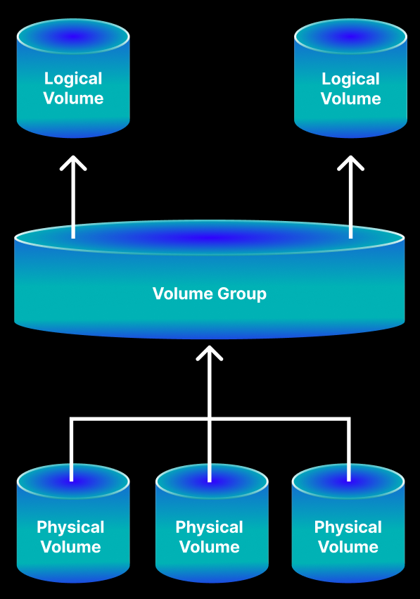
As stated in the technical definition, LVM creates an abstraction layer over physical storage. As you can see below, this layer consists of 3 components.

Physical Volume

It is the lowest layer of the LVM structure. It’s created when a physical storage unit, such as a disk, partition or RAID array is made usable by LVM. In order for a physical disk to be used by LVM, it must be converted into a Physical Volume first.

Volume Group

The LVM combines these storage devices that have already been made into physical volumes to form a pool of storage space known as a volume group. Physical volumes cannot be accessed individually; they must first be pooled together in a volume group, and by doing this, the capacities of physical volumes having different sizes are combined together into a logical pool of storage space.

Logical Volume

It’s the highest layer of the LVM structure. It’s a section carved out of the Volume Group at a specific size, according to need. Logical Volumes behave similarly to classic disk partitions, and a file system can be set up on them, formatted, and mounted. Unlike a physical disk, the size of Logical Volumes can easily grow or shrink based on the capacity of their Volume Group. As can be understood from the situation I described earlier, this is one of LVM’s biggest advantages.

Now that I’ve covered these definitions, I’ll continue by explaining the remaining details through an LVM configuration scenario, without burying you in more technical information. For your convenience and mine as we move through the rest of the article, I recommend familiarizing yourself with these terms:

PV: Physical Volume

VG: Volume Group

LV: Logical Volume

LVM Configuration Scenario

Now that I’ve explained LVM and its structure, I’ll walk through an LVM configuration using a scenario to better illustrate the topic. Our scenario is as follows:

There are 2 newly added disks in the system, 50 GB and 100 GB in size. As a solution to the “log files filling up the disk” problem I mentioned earlier, we decide to manage these disks with LVM. We’ll first convert these disks into PVs, and then bring them into LVM. Next, we’ll combine these PVs into a common pool called a VG. From this pool, we’ll create two LVs, lv_data1 at 25GB and lv_data2 at 50GB, and after setting up a file system on each, we’ll mount them at /data1 and /data2.

After completing the setup, we’ll simulate the “log files filling up the disk” scenario again on /data1. As a solution, we’ll directly grow the size of our LV by using the free space in the VG that the LV belongs to.

After that, we’ll fill up the free space on /data2 as well. When we want to expand this LV’s size to 150G, we’ll see that there’s no free space left in the VG.

To solve this problem, we’ll add a 3rd disk to the VG to expand the pool, and then grow /data2. Next, assuming that the disk lv_data1 resides on has started to fail, we’ll migrate lv_data1 to another disk. After completing these steps, I’ll go on to show LVM’s other features.

LVM Configuration with Explanations

First, let’s view the new disks using the lsblk command. Before turning the physical disks into PVs, there is one more thing I have to mention. It is possible to use the physical disks without partitioning and add them directly to LVM. Moreover, it is possible to partition the disks and use partitions as physical volumes when adding them to LVM. But, according to Red Hat Documentation website, it is better to partition the disk and make one partition covering the whole disk, mark it as Linux LVM, and then convert this partition into PV ². That is why I will follow Red Hat’s recommendations instead of working with the disks directly. Now that I’ve explained this detail, we can continue.

Disk Partitioning

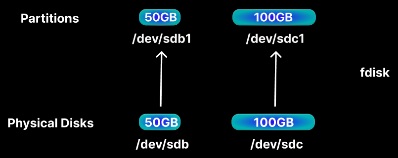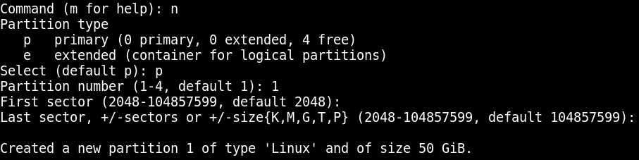
You can see the process we’ll perform below. At the beginning of each section, I’ll include these diagrams to make it easier to follow and explain. First, we’ll use the fdisk command to partition the newly added disks into a single partition each, and mark them as Linux LVM. Run the fdisk /dev/sdb command, then type n to begin creating a new partition. 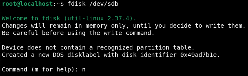Now type p to select the primary partition option. For the Partition number, enter 1. Since we’ll be using the entire disk for this partition, you can leave the First sector and Last sector options blank and press enter to skip them. 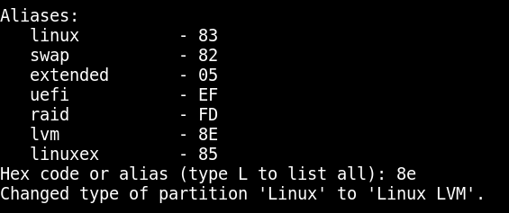Type t to mark the partition as Linux LVM. Type L to see the options. Mark the partition as Linux LVM using the hex code 8E. 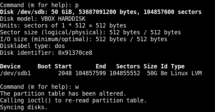Check the changes you’ve made by typing p, then type w to save and exit. 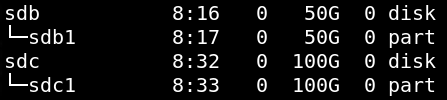Repeat this same process for /dev/sdc. The disks should look like this:

Converting Physical Disk Partitions into Physical Volumes

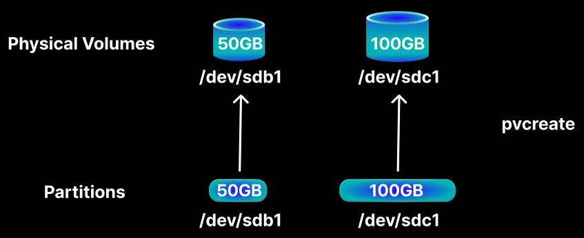We use the pvcreate command to create a Physical Volume (PV). To convert the partition into a PV for use in LVM, run the pvcreate /dev/sdb1 command. Use the pvdisplay command to view the details of the PV we created. 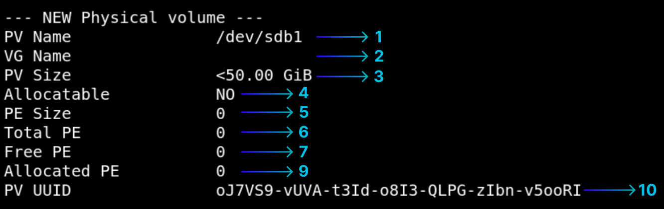1: The PV’s name is /dev/sdb1, the name of our partition that we used to create the PV.

2: VG Name is empty because we haven’t added this Physical Volume to a Volume Group yet.

3: PV Size 50 GiB indicates the size of the Physical Volume. Don not confuse GiB here with GB. You can find the difference between them in the references³ section.

4: Allocatable NO because the Physical Volume hasn’t been added to a Volume Group yet.

5 - 6 - 7 - 8: Let me explain what PE means in this part. PE (Physical Extent) is the smallest unit of storage on the Physical Volume (PV). After the addition of Physical Volume to a Volume Group, the hard drive is not managed in bytes but is divided into extents with fixed size. The standard size of extents is 4 MiB. Therefore, our Physical Volume is not yet added to a Volume Group and thus isn’t divided into extents and that is why all fields connected to PE have 0 value now.

9: This is the Unique Identifier of the Physical Volume. The UUID is stored in the metadata of the LVM located in the header of the disk such as /dev/sdb1. In simpler terms, the UUID is not stored on the side of the OS, but physically stored in the disk itself. Regardless of the changes in the names and order of the disks or even the movement to a different server, the PV UUID stays the same. The LVM hierarchy or the association of the PV, VG, and LV is done through the cross-reference using the UUIDs. Now let’s continue by converting the /dev/sdc1 partition into a Physical Volume.

pvcreate /dev/sdc1 Use the pvs command to view a summary of the PVs we’ve created. Our disks are now ready to be used by LVM and to create a VG.

Creating a Volume Group from Physical Volumes

Now we’ll use one of the PVs we created along with the vgcreate command to create a VG. After that, we’ll add the other PVs to this pool.

Syntax: vgcreate <vg_name> <pv_path>

Command: vgcreate vg_base /dev/sdb1 Before we start examining the VG, let’s take another look at the details of the /dev/sdb1 PV we just created. 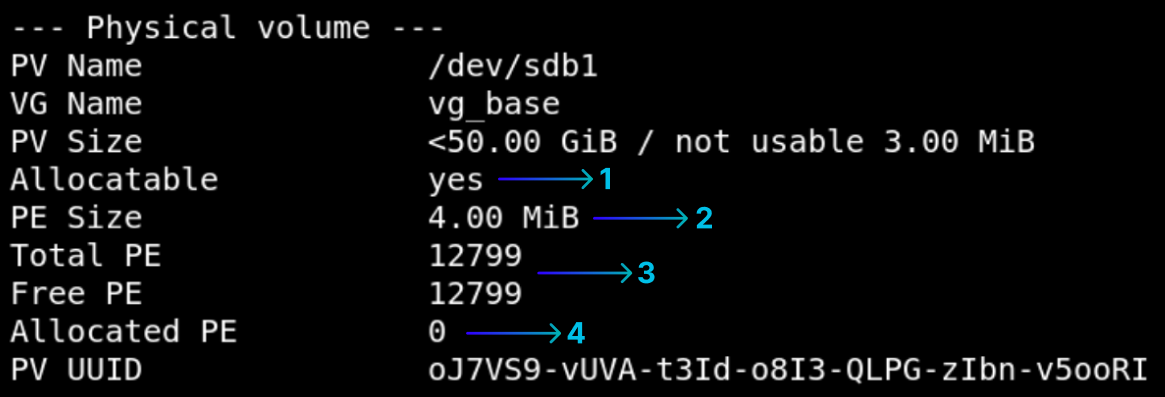1: The PV is now allocatable since it’s part of a VG.

2: As I explained earlier, once the PV is added to the VG, it gets divided into 4 MiB blocks.

3: This shows that the PV consists of a total of 12799 4 MiB blocks, and indicates the free space.

4: No space has been allocated from this disk yet. We can better see the difference by comparing our two PVs. 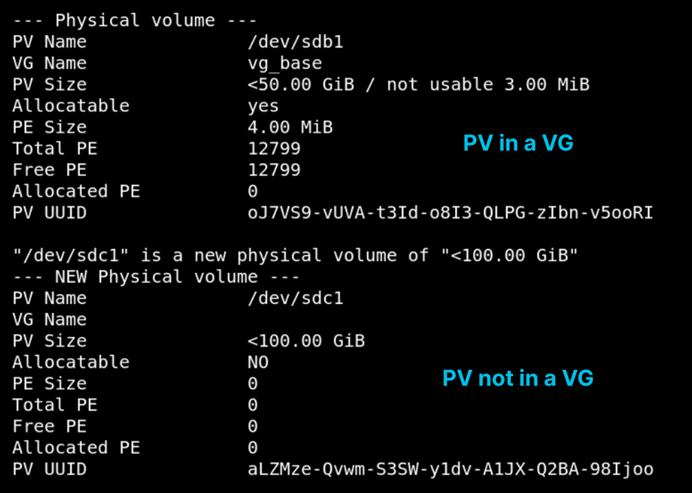As you can see, after being added to the VG, the PV /dev/sdb1 has been divided into 12799 blocks of 4.00 MiB in size. The PV /dev/sdc1, on the other hand, hasn’t been divided into blocks yet since it hasn’t been added to a VG. Now let’s examine the VG we created using the vgdisplay command. 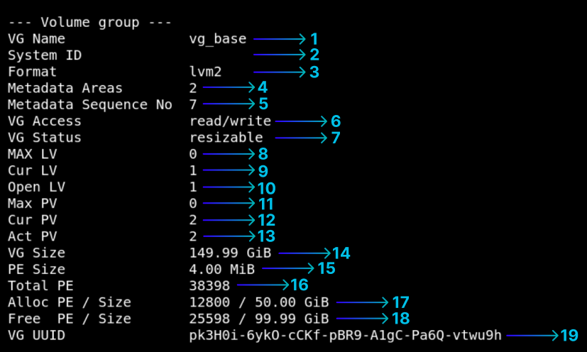1: The name of the VG.

2: The system ID of the group. Usually used in cluster environments, so it’s empty.

3: The standard LVM format version.

4: Configuration data of the VG is called metadata. The metadata contains configuration data such as which size does an LV have in LVM, where PEs are located, UUIDs, names, etc. By default, the metadata is stored by copying it into the metadata⁴ areas of all PVs of the VG. I don’t want to talk about this topic in more detail than needed. You can look in the sources section for further info.

5: A revision number that increases by 1 every time an operation is performed on the VG.

6: By default, creating, deleting and resizing of the LVs is possible. If it is set to “read-only” then it is not possible to perform any operations like creating, deleting and resizing the LVs.

7: A fixed value marked as resizable. It rarely changes except in very rare cases, so I won’t go into detail about it.

8: The number of LVs that can be created within the VG. A value of 0 means unlimited.

9: The number of LVs within the VG. It’s 0 because we haven’t created any LVs yet.

10: The number of LVs currently in use is 0.

11: The number of PVs that can be added to the VG. A value of 0 means unlimited.

12: The number of PVs in the VG.

13: The number of active PVs in the VG.

14: The VG’s size in GiB. This value will increase shortly once we add our other PV, /dev/sdc1.

15: The PE (Physical Extent) size. 4 MiB by default.

16: Indicates that the VG consists of 12799 blocks of 4 MiB.

17: The number of allocated blocks and gibibytes. It’s 0 since we haven’t created an LV yet.

18: The number of allocatable blocks.

19: The unique identifier number. As I explained earlier, when we add a PV to a VG, LVM writes the VG’s UUID onto that PV. This way, it knows which VG it belongs to by its UUID, not by the PV’s name.

As you can see here in the output of the pvs -o pv_name,pv_uuid,vg_name,vg_uuid command, /dev/sdb1 points to the vg_base group via its UUID. Now let’s add the /dev/sdc1 PV to the VG we created, using the vgextend command.

Syntax: vgextend <vg_name> <pv_name>

Command: vgextend vg_base /dev/sdc1 Using the vgdisplay command again, we can see that the VG’s size has increased. The Cur PV and Act PV counts have gone up to two. 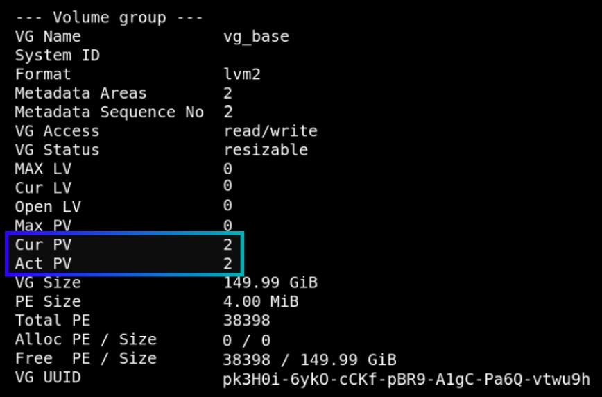Now our PVs are in the same pool. The PV UUIDs point to the VG UUID of our VG named vg_base.

Creating Logical Volumes from the Volume Group

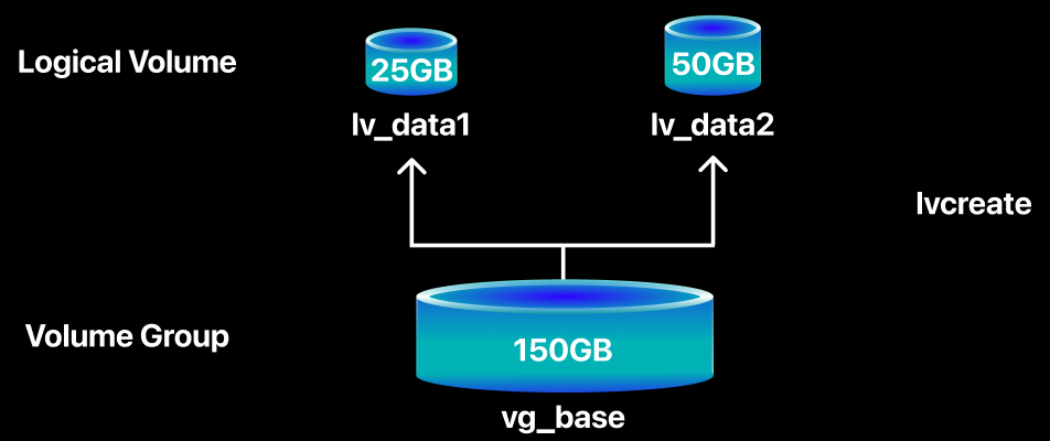Now, we’ll use the lvcreate command to create a Logical Volume (LV) from our VG named vg_base, on which we can create a file system.

Syntax: lvcreate -L <size>[M|G|T] -n <lv_name> <vg_name>

Command: lvcreate -L 25G -n lv_data1 vg_base

With this command, we specify the amount we want as a size (M, G, T) using -L, or as a percentage or in blocks using -l. Although it’s usually not specified in blocks, it’s still useful to know. After specifying the name of the LV we want to create with -n, we indicate which VG this volume will be created from. You can examine the LV we created using the lvdisplay command. 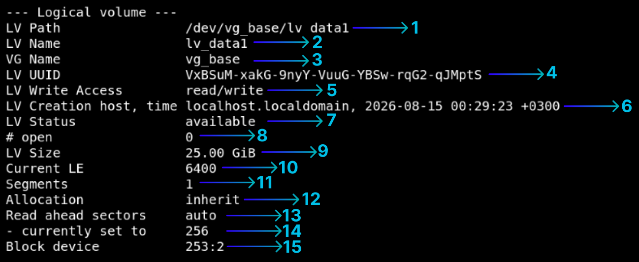1: The device path for the LV. Once the file system has been added, this path will be used to mount the LV.

2: The name of the LV.

3: The name of the Volume Group that the LV belongs to.

4: Unique ID number for each LV on the system.

5: Read/write access is enabled on the LV. You may set the LV to read-only access.

6: Information regarding which host the LV has been created and when.

7: The LV is online and available for use.

8: The LV is online and not mounted. No user is accessing it.

9: Size of the LV.

10: Number of Logical Extents (Logical Blocks) required by the LV. The LV is made up of 6400 blocks of 4 MB in size.

11: Shows how many segments the LV consists of. On disk, it’s a single, unsplit segment. I’ll explain this part later.

12: Allocation rules, taken from the VG, meaning there’s no special setting. This is generally the case.

13: The read-ahead setting is set to automatic.

14: The actual current “read-ahead” value under the automatic setting, 256 sectors. Not an important detail.

15: Shows the major:minor number within the kernel. An identifier assigned at runtime at the kernel level. Again, not an important detail in our case.

Now let’s create the 50GiB lv_data2 LV. lvcreate -L 50G -n lv_data2 vg_base Let’s examine the current state of our VG using the vgdisplay command. 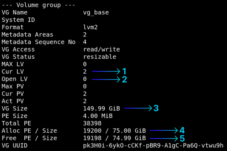1: The number of LVs in the VG.

2: Shows how many of the LVs are open/in use. It’s 0 for now, since we haven’t added a file system to the LVs we created and mounted them yet.

3: The total size of our VG. We had added 2 PVs, 50 and 100GiB.

4: 75GiB of this 150GiB pool is being used. We created 2 LVs, 25 and 50GiB.

5: The remaining free space in the VG.

We can see the distribution using the lsblk command. 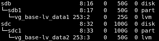As you might notice here, by default, LVM doesn’t select a PV randomly or sequentially when creating an LV. Instead, it selects the PV that’s the best fit for the size of the LV to be created. For example:

The 25GiB LV > was created from the 50 GiB PV. The 50GiB LV > was created from the 100 GiB PV.

In other words, rather than first filling up one PV completely and then splitting the overflow onto another PV (the segment topic I’ll explain later), LVM selects, among the PVs in the VG, the most suitable one that can hold the LV as a single piece. LVM uses the normal allocation policy by default when allocating physical extents for an LV. According to Red Hat’s official documentation ⁵, it’s recommended that you not change this setting.

If we had created a 125 GiB LV, since there’s no PV of that size, the LV would normally have been split into segments, as you can see below. 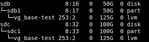Let’s take a look at this LV that I created as an example, using the lvdisplay command. 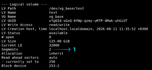1: I said that I would explain this part later. The Segments field shows how many pieces our LV consists of. As you can see above, since no PV in our VG is 125GiB in size, our LV has been divided into 2 parts. An LV doesn’t have to be physically contiguous; it can be fragmented like this. Each contiguous portion is called a segment. If the segment count is 1, it means the LV resides as a single piece in a contiguous area. This is the preferred, clean layout.

If the number of segments is greater than 1, this signifies that the LV is distributed in multiple PVs. In scenarios such as this, when the size of the PVs isn’t large enough, it becomes natural for LVs to be partitioned into segments. But, as we well see in another example, this kind of fragmented structure isn’t preferred when working with HDDs.

Creating and Mounting a File System

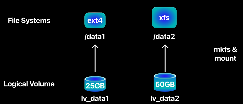At the end of the LVM process, we can start using our LVs by adding a file system with the mkfs command and mounting them onto the system. Syntax: mkfs.<filesystem_type> <device_path>

A quick reminder before creating the file systems, the ext4 file system is ideal for desktop use or small-sized systems. Its size can be shrunk.

The xfs file system’s size can’t be shrunk. In other words, you can grow the size of an LV, but if you want to shrink it, you’ll need to delete the LV and recreate it from scratch. So you should be careful about this.

Now let’s create the file systems.

Command 1: mkfs.ext4 /dev/vg_base/lv_data1

Command 2: mkfs.xfs /dev/vg_base/lv_data2

After creating the file systems on our LVs, let’s verify with the blkid command.

Command 1: blkid /dev/vg_base/lv_data1

Command 2: blkid /dev/vg_base/lv_data2 Let’s create the mount points.

Command 1: mkdir /data1

Command 2: mkdir /data2

Let’s mount our LVs to these mount points.

Command 1: mount /dev/vg_base/lv_data1 /data1

Command 2: mount /dev/vg_base/lv_data2 /data2

Let’s use the lsblk command to check. 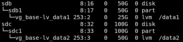Now the LVs are ready to be used. To make the mount points persistent, we’ll add the LV UUIDs to the /etc/fstab file. Let’s use the blkid command to find out the UUIDs of our LVs. Copy the UUIDs and add them to the bottom of the /etc/fstab file, as shown below. Now, every time the system boots, our LVs will automatically be mounted to these folders. Now that we’ve completed the LVM process, you can see all the steps we performed below.

Disk Filling Up Scenario: /data1

Now we’ll simulate the “log files filling the disk” scenario again on /data1. The command we’ll use for this test: cat /dev/zero > /data1/application_1.log

You can see the LV filling up.

Now that we’re using LVM in our system, we can solve this problem by expanding the size of our storage space. The command used to expand LV size is lvextend

Syntax 1: lvextend -l +100%FREE <lv_path> uses all the free space in the VG.

Syntax 2: lvextend -L 50G <lv_path> expands the LV to a specific size.

Syntax 3: lvextend -L +50G <lv_path> adds a specific amount to the LV.

Now let’s expand the size of our LV. Command: lvextend -L +24G /dev/vg_base/lv_data1 I used 24G instead of 25G because lv_data1 resides on the 50GiB PV /dev/sdb1. At first you might think of using the entire 50GiB PV by adding 25GiB more to the LV. However, the allocatable size of /dev/sdb1 for LVM isn’t exactly 50GiB, it is approximately 49.5GiB. In other words, if I had expanded it by 25GiB instead of 24GiB, we would have seen the remaining 500 MiB split off onto another disk (segment). As you can see below, this causes unnecessary complexity and makes management harder. 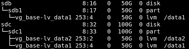So, if you don’t want your LV to be split onto other disks beyond the PV it currently resides on when expanding it, pay attention to this situation.

Let’s check the size of our LVs using the df -h /data1 /data2 command. As you may have noticed, even though we added 24GiB more to the LV, its size didn’t increase, and it still shows as 25GiB instead of 49GiB. This is because the lvextend command just expands the size of the LV but does not do anything to the file system. Therefore the next step is to expand the file system too. The commands to be used here are:

To expand the XFS file system: xfs_growfs To expand the EXT4 file system: resize2fs

Let’s expand the file system of our LV.

resize2fs /dev/vg_base/lv_data1 Let’s check the size again using the df -h /data1 /data2 command. As you can see, after expanding the file system, our LV’s size increased to 49GiB.

Disk Filling Up Scenario: /data2

In this part, just like we did with /data1, we’ll fill up the free space on /data2 as well. This time, we want to solve the disk-filling problem by growing the size of the lv_data2 LV to 150GiB. However, there isn’t enough space left in our VG. That’s why we’ve added a new disk to the system, and we’ll expand the size of the VG. We’ll set our LV’s size to 150GiB, and finally complete the process by expanding the file system as well.

We’ll use the commands you already know from previous sections and follow the same steps. The purpose of this example is to show the process of growing our LV’s size when there’s no free space left in the VG.

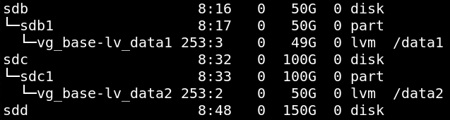
Now let’s fill up the free space using the cat /dev/zero > /data2/application_2.log command. We want to expand the size of lv_data2, which /data2 is mounted on, to 150GiB, but as you can see here, there’s only 50GiB of space left in the VG. 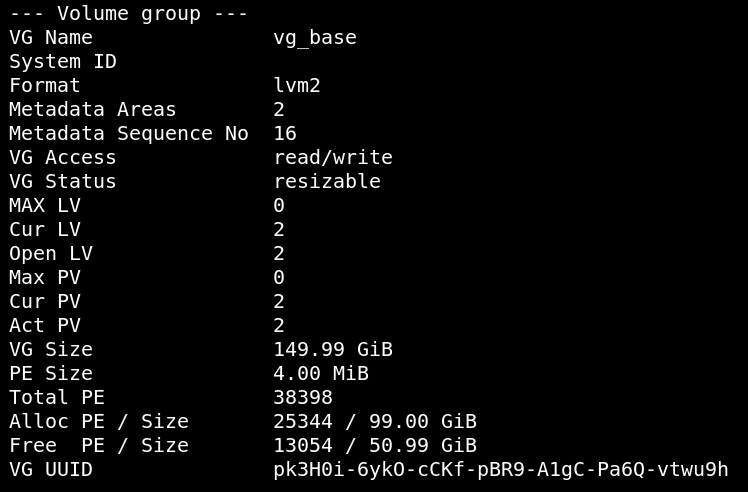To solve this problem, we’ve added a 150GiB /dev/sdd disk to our system, and we’re verifying it using the lsblk command. 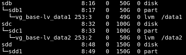Before converting our disk into a PV to use in the VG with the pvcreate command, as you’ll recall, we first create a partition that spans the entire disk. This is the same process I explained in the earlier sections. So I won’t show the disk partitioning step again. If you’d like, you can review the steps again by clicking on “Disk Partitioning” in the “Contents” panel.

As you can see below, we’ve created a partition that spans the entire disk. Now let’s convert this partition into a PV.

pvcreate /dev/sdd1 We’re growing our VG’s size by adding the PV we created, using the vgextend command. As a reminder:

Syntax: vgextend <vg_name> <pv_path>

Command: vgextend vg_base /dev/sdd1 Let’s take a look at our VG’s new size using the vgdisplay command. 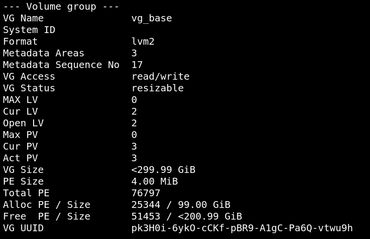After adding our new PV, the total space has increased from 150 GiB to 299.99 GiB. We can now use this space to grow the size of our lv_data2 LV.

Command: lvextend -L 150G /dev/vg_base/lv_data2 I mentioned that after growing our LV’s size using the lvextend command, we need to expand the file system. We shouldn’t use the resize2fs command we used in the previous stage, because lv_data2 uses the XFS file system. You can find out the file system type using blkid. That’s why the command we will use is: xfs_growfs

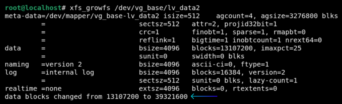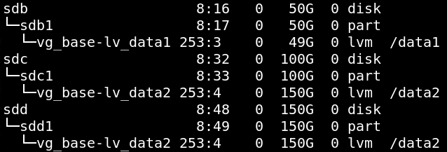
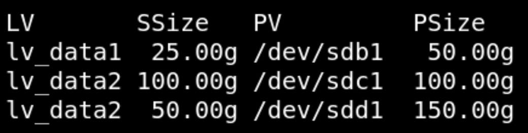
xfs_growfs /dev/vg_base/lv_data2 We’ve expanded the XFS file system. You can see that the size of /data2 has increased. Our current state looks like this with the lsblk command. Since a single PV couldn’t accommodate the lv_data2 LV that we expanded to 150 GiB, this LV is now spread (segmented) across the /dev/sdc1 and /dev/sdd1 PVs. It’s not possible to tell from the standard lsblk or vgs output how much space lv_data2 takes from which PV. You can use this command to find this out: Command: pvs -o lv_name,lv_size,pv_name,pv_size,seg_size --units g -S "lv_name=lv_data2" Although the command we used isn’t very practical, its output is quite easy to understand.

1: The LV’s name and size.

2: The PVs this LV resides on, and their sizes.

3: The total space this LV takes from these PVs.

In other words, the 150GiB LV lv_data2 uses 100GiB of space from the 100 GiB /dev/sdc1, and 50GiB of space from the 150 GiB /dev/sdd1.

Shrinking a Logical Volume’s Size

We decide that we no longer need 24GiB of the space on the 49GiB lv_data1 LV. So we’ll shrink our LV’s size to free up room in our VG for other LVs. Before we begin, there are two important details you need to know. In LVM, shrinking an LV’s size is riskier than growing it, because there’s a risk of data loss. The file system must be shrunk first, and then the LV. If you do this in the reverse order, you’ll lose your data. The other detail is that the XFS file system doesn’t support shrinking in any way. XFS can only be grown. If you’re using XFS, the only way to shrink an LV is to create a new LV at the size you want and migrate your data there. That’s why we’ll shrink lv_data1, which uses the EXT4 file system.

First, let’s start by unmounting lv_data1.

Command: umount /dev/vg_base/lv_data1

Let’s check our file system for errors.

Command: e2fsck -f /dev/vg_base/lv_data1

Let’s shrink our file system.

Command: resize2fs /dev/vg_base/lv_data1 25G Now we can shrink our LV.

Syntax: lvreduce -L <target_size> <lv_path> Command: lvreduce -L 25G /dev/vg_base/lv_data1

Let’s mount it again and check.

Command 1: mount /dev/vg_base/lv_data1 /data1

Command 2: df -h | grep data

As you can see, it’s a short and simple process. But be careful not to mix up the order, or you could lose your data.

Disk Failure Scenario

Now, let’s consider a situation where the /dev/sdb disk, which contains the lv_data1 LV mounted at /data1, starts to fail. The first solution that comes to mind might be to set /data1 to read-only, as many people suggest, and start the migration using the mv command. However, as you might know, this causes downtime. Also, mv operates at the file system level, so if something like a power outage or a disk failure occurs during the transfer, it has no way to resume or roll back the operation. You will have to handle it manually and figure out which files were transferred and which weren’t. Also, if there are several LVs on the disk, moving files with mv won’t remove the disk from the VG, so the other LVs will remain on the failing disk.

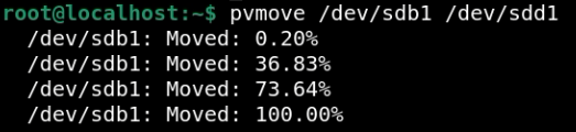
For that reason, before we proceed to remove our faulty disk from the VG, we will use the pvmove command to relocate the LV and the data in it safely. Unlike mv, the pvmove command works on the block level. To put it simply, it doesn’t really care what file system it is and what files it contains. The pvmove command relocates PEs belonging to an LV from one PV to another. It is not a file relocation but relocation of the LV itself. It does it in segments creating a temporary mirror (similar to RAID) between the source and the destination. The process progresses in small segments and each time when one is finished, it creates a checkpoint in the VG metadata. The process takes place in the background while the LV is mounted and working. So, there is no need to unmount your disk and stop all services to move the data. If the system crashes or the disk throws some errors while you are doing this, LVM will mark it as an unfinished pvmove operation and the next time you use the command again, it picks up where it left off, because LVM knows which PEs have been moved and which haven’t. This way, everything is preserved. Now that I’ve explained these details, we can begin.

We’ve noticed that the /dev/sdb disk has started to fail. We had created the PV named /dev/sdb1 on this disk. That means all the LVs and data on the /dev/sdb1 PV are at risk. So we want to safely migrate these LVs to the /dev/sdd1 PV, which we created from our newly added /dev/sdd disk. First, let’s check whether there’s enough space on /dev/sdd1 using the pvs command. As you can see, the /dev/sdd1 PV has enough space. Before we begin, let’s see which LVs are using which PVs, so we can refer back to it later, using the command pvs --segments -o lv_name,seg_size,pv_name,pv_size --units g | awk 'NF==4' As a best practice, let’s back up our VG’s LVM configuration information using the vgcfgbackup vg_base command. Now let’s begin the process using the pvmove command.

Syntax: pvmove <source_pv> <destination_pv>

Command: pvmove /dev/sdb1 /dev/sdd1 After the migration completes, let’s take another look at the current state using the pvs --segments -o pv_name,pv_size,lv_name,seg_size --units g command again. As you can see, the lv_data1 LV has now been moved to the /dev/sdd1 PV. After the migration is complete, we can remove the /dev/sdb1 PV, created from the failing disk, from the VG. The command we’ll use is vgreduce. Syntax: vgreduce <vg_name> <pv_name> Command: vgreduce vg_base /dev/sdb1 Now that we’ve removed our PV from the VG, we can remove our disk from PV status using the pvremove /dev/sdb1 command. We’ve now completed our operation, and without unmounting the disk or switching it to read-only mode, we migrated all the LVs on the disk and their data live, without any downtime. If we had had more than one LV, the same steps would still apply.

LVM Striping

Before I get into the topic of LVM striping, I should mention creating RAID using LVM. After converting your physical disks into PVs, you can use LVM’s RAID feature to create RAID at levels 0, 1, 4, 5, 6, and 10 from your PVs⁶. However, common practice recommends creating the RAID first, and then adding this RAID device to LVM as a PV. In other words, rather than managing disk-failure handling and redundancy tracking with LVM, it’s a more correct approach to create the RAID using the mdadm command, which is designed specifically for this purpose. This way, RAID management is handled by mdadm, while volume management is handled by LVM.

For this reason, instead of covering LVM’s RAID features comprehensively in this section, we’ll focus on the RAID 0 (striping) method, which doesn’t provide redundancy but is the most commonly preferred use case within LVM. It’s used to increase disk performance.

We’ve added 2 disks to our system: /dev/sde at 50GiB and /dev/sdf at 50GiB. We’ll convert these disks into PVs, add them to LVM, and create an LV with a RAID 0 (striping) configuration.

First, let’s take a look at our disks. Let’s partition our disks in order to create PVs. You can review this process in the “Contents” section under “Disk Partitioning.” The output of the lsblk /dev/sde /dev/sdf command should look like this: We’re creating our PVs using the pvcreate /dev/sde1 /dev/sdf1 command. To make things easier to track, we’ll create a new VG named vg_stripe, separate from the vg_base VG that we created in the earlier stages. As a reminder:

Syntax: vgcreate <vg_name> <pv_path>

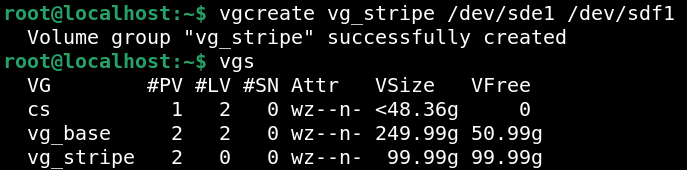
Command: vgcreate vg_stripe /dev/sde1 /dev/sdf1

After running this command, let’s check our VG using the vgs command. Now we’ll create a new LV named lv_stripe with a RAID 0 configuration, using all of the free space in the vg_stripe VG.

Syntax: lvcreate --type <raid_type> -i <stripe_count> -I <stripe_size> -l <lv_size> -n <lv_name> <vg_name>

Command: lvcreate --type raid0 -i 2 -I 64 -l 100%FREE -n lv_stripe vg_stripe --type raid0: Specifies the type of LV to be created.

-i 2: The stripe count. Specifies how many physical disks/PVs the data will be split across. The data will be distributed sequentially across 2 PVs, /dev/sde1 and /dev/sdf1.

-I 64: Specifies the stripe size. In other words, a stripe size of 64 KiB means that once 64 KiB of data is written to one disk, writing moves on to the next disk.

-l 100%FREE: The space to be allocated to the LV. That is, we’re using all of the space in our vg_stripe VG.

-n lv_stripe: The LV’s name.

vg_stripe: The source VG the LV will be created from.

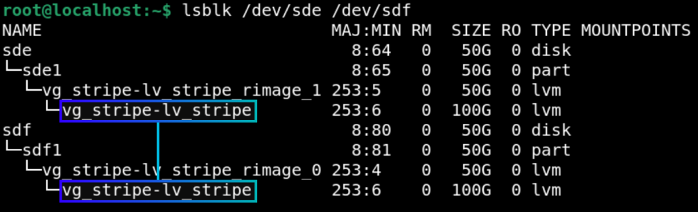
After creating our LV, let’s examine lv_stripe using the lsblk /dev/sde /dev/sdf command. Our LV named lv_stripe, 100GiB in size, is distributed across 2 physical disks in a RAID 0 configuration. The rimage_0 and rimage_1 you see above are the sub-LV components that LVM RAID creates for each stripe/disk. They aren’t something that requires direct intervention, so we don’t need to go into their details.

Let’s create a file system on lv_stripe.

Command: mkfs.xfs /dev/vg_stripe/lv_stripe

To be able to use our LV, let’s create a mount point and mount it there: Command 1: mkdir /striped

Command 2: mount /dev/vg_stripe/lv_stripe /striped 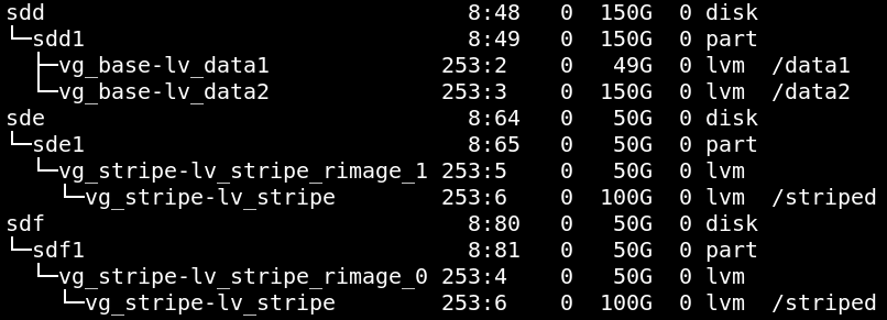Our LV named lv_stripe is mounted to the /striped directory and we can start using it now. Don’t forget to add an entry to the /etc/fstab file to make it persistent.

Next, let’s compare lv_data1 which exists on /dev/sdd1 to our new lv_stripe in terms of write speed to show the performance benefit of RAID 0 (striping).

There’s an important point I need to mention here. If you’re performing this on a virtual machine like I did, you won’t see the write speed difference in the fio test. This is because the disks we added to the VM are virtual. This means in the background they are sharing the host machine’s single physical disk. Even though we correctly set up the RAID 0 configuration at the LVM level, they don’t provide true parallelism because these virtual disks physically exist on the same underlying disk. This is why we can’t measure striping’s real performance benefit in a VM environment. In a scenario where we’re not using a VM, the difference between the two LVs in the fio test would look like this: lv_data1’s write speed. lv_stripe’s write speed. As you can see, write speed roughly doubles on average. It is important to note that RAID 0 doesn’t provide redundancy. In cases where redundancy is needed, you should use one of the RAID 1, 4, 5, 6, or 10. Explaining all the RAID levels would make this article for too long so I wanted to demonstrate LVM’s RAID support using only the striping configuration. You can check the references section for details on the other levels.

LVM Snapshots

As stated on the Red Hat documentation site, LVM’s snapshot feature makes it possible to create virtual images of a device at a particular point in time, without causing any service interruption. After a snapshot is taken, when a change is made to the original (origin) device, the snapshot feature creates a copy of the changed data area as it was before the change; this way, the device’s previous state can be reconstructed.⁷

The most important thing to know about snapshots is that they aren’t a backup method. A snapshot lets you roll back to a state at a particular point in time. But this isn’t because we copy all of the data. What we actually do is copy the changes that occur to the original data over time. This process is called “COW,” or “Copy on Write.” Before a change is made to an LV, the unmodified/original version of the data that is about to be changed is copied to the snapshot area, and then the actual change is carried out on the original data. Later, when we want to “roll back” from this snapshot, these original blocks stored in the snapshot area are written back onto the original LV, and this is how we perform the “rollback.” So this is why snapshots aren’t a backup method. They don’t hold all the data, they only hold the difference. You can see this process in the amazing animation I made below.

As you can see, the reason why snapshots cannot be used as a way of creating backups is that they do not contain all the information, but only the difference. Moreover, since the snapshot is located in the same Volume Group as well as on the same physical disks as the original LV it is created from, any failure of such disk would result in losing both the original LV and the snapshot.

The COW process impacts write performance. This effect is only felt once when the block is changed the first time because if the same block is changed later on, the original content in the block has already been duplicated in the snapshot. But if there are multiple snapshots available, then the process is repeated for all of them, and performance drops even further.

There are two ways to take an LVM snapshot: Thick provisioning and Thin provisioning. Thick provisioning is the classic and older methed. In this method, at the moment of creating a snapshot, the snapshot size is estimated and allocated right away from the VG. Regardless of the data that is written to it, the space in the VG will be considered allocated and will not be accessible for other LVs. The changes are recorded till the storage of the snapshot is full. When the storage of the snapshot becomes filled up to a certain level, a message is logged into the system log. If you ignore this message and fully fill the storage of the snapshot, the snapshot will become invalid, as it will no longer be able to record the changes made in the origin volume.

Thin provisioning, on the other hand, is completely different from the classic thick provisioning. This is based on the idea of provisioning space for the LVM “only as much as is actually used.” The size of the space does not have to be predefined when making a snapshot. Instead of defining the space that should be allocated in advance for the snapshot, thin pools are created first, and then the snapshots allocate as much space from those pools as needed depending on what changes happen in the origin volume. This way, taking a snapshot takes up almost no space at the start.

However, there are some downsides to it. While thick provisioning creates dedicated space for each individual snapshot, thin provisioning shares a single storage space among all the snapshots. This means that in thick provisioning only the designated snapshot is required to be monitored but in thin provisioning, the entire storage space needs to be monitored. If the pool fills up completely, write operations may fail for all LVs and snapshots tied to that pool.

I’ll demonstrate the LVM snapshot creation process using the classic thick provisioning method. To avoid making this article longer than necessary, and to cover it in more detail, I’ll explain the thin provisioning method in a separate post.

Let’s take a look at our LVs using the lvs command. 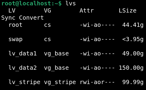The lv_data1 LV is 49 GiB in size and belongs to the vg_base VG. We want to create a 10GiB snapshot of this LV. As you know, when we create a snapshot using the thick provisioning method, the space is allocated immediately. So we first need to check the free space in our VG. 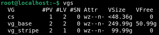As you can see, vg_base is suitable for creating a 10GiB snapshot. Now let’s find out lv_data1’s mount point using the lsblk /dev/vg_base/lv_data1 command. First, let’s take a look at the current data at this mount point using the ls and cat commands, so we can compare it with the changes we’ll make later.
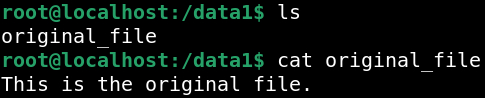
We have a file named “original_file” in /data1. Shortly, after creating a snapshot of our LV, we’ll change this file’s content and add a new file.

Now we can create a snapshot of the lv_data1 LV. Before we start, you should know that a snapshot is a special LV type in LVM. There’s no separate, dedicated command for taking a snapshot, because a snapshot is also treated as an LV under LVM management. So the command we’ll use is lvcreate.

Syntax: lvcreate -L <size> -s -n <snapshot_name> <origin_lv_path>

-L: The size of the LV to be created (in this case, the snapshot’s COW area).

-s: The snapshot flag. Tells LVM that this LV will be a snapshot, not a regular LV.

-n lv_data1_snap: The name to be given to the snapshot being created.

/dev/vg_base/lv_data1: The origin volume, i.e., the full path of the actual LV the snapshot is being taken of.

Command: lvcreate -L 10G -s -n lv_data1_snap /dev/vg_base/lv_data1 Now let’s take another look at our LVs using the lvs command again. 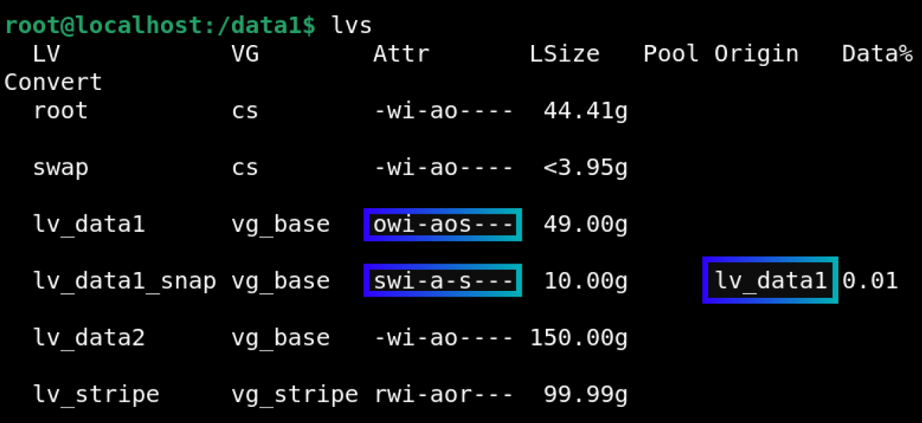We’ve created a snapshot of the lv_data1 LV. The “o” you see in the Attributes column indicates the origin LV, while the “s” indicates the snapshot LV. As you can see in the Origin column, lv_data1_snap points to lv_data1. (The “r” you see for lv_stripe indicates the RAID configuration that we made before.)

For our snapshot to record the changes we make to the origin volume, we need to mount it.

Let’s create the mount point.

mkdir -p /snapshot

Let’s mount our snapshot to this point.

mount /dev/vg_base/lv_data1_snap /snapshot

Let’s take a look at lv_data1_snap’s content using the same commands. As you can see, the data in /data1 (i.e., in the origin LV lv_data1) appears the same way in our snapshot too. Don’t let this mislead you though. Because as you know, the “original_file” we see in the snapshot isn’t actually a copy stored in the snapshot’s own space. It only appears because the read request is redirected to /data1. The moment we make a change to the origin, the COW mechanism will kick in, and the old version of the block about to change will be copied to the /snapshot area before being overwritten. Now we’re making a change to the “original_file” file on /data1. After making this change, “original_file” has now truly become a copy stored in the snapshot’s own space. It’s not redirecting the read request and showing the data now. Don’t let the fact that I changed both the name of the “original_file” file and its content in this example make you think LVM snapshot operates at the file level. LVM snapshot doesn’t operate at the file level, but at the block level. I used this approach so you could clearly see the difference and follow along more easily.

We can now perform a rollback from the LVM snapshot using the lvconvert command. We have to unmount the origin and the snapshot first.

Command 1: umount /data1

Command 2: umount /snapshot

After this, we can begin the rollback process.

Syntax: lvconvert --merge /dev/<vg_name>/<snapshot_LV>

Command: lvconvert --merge /dev/vg_base/lv_data1_snap

After the process, let’s mount the origin again.

Command: mount /dev/vg_base/lv_data1 /data1 Let’s run the lvs command to view our LVs. 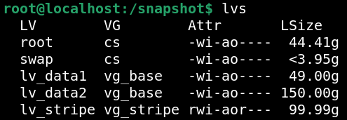Our snapshot named lv_data1_snap no longer exists, because once the merge operation completes, our snapshot is automatically deleted.

With that, we’ve reached the end of this post. As my first post, I tried to cover the topic of LVM in as much detail as I could. I’m aware there are some details I didn’t get into fully, in order to keep the article from running longer than necessary and to make it easier to follow. I’ll cover these details more deeply in my future LVM posts. You can find the sources I used below. Thanks for reading.

References